• Skip navigation
  • Skip to navigation
  • Skip to the bottom
WiN-Lab
Suche öffnen
  • Deutsch
  • zur Forschungsgruppe Netz am RRZE

WiN-Lab

Navigation close
  • Quantum Technology
    • Basics
    • Quantum Computing
    • Quantum Key Distribution
    • Quantum Networks
    • Quantum Simulation
    • Quantum Initiatives
    • Tutorials
    • Additional Information
    zu Quantum Technology
  • Projects
    • WiN-Lab Projects
      • Current WiN-Lab Project
      • Closed WiN-Labor Projects
    • Cooperation Projects
      • Current Cooperation Projects
      • Completed Cooperation Projects
    zu Projects
  • Publications
  • Archive

WiN-Labor

blogdescription

In page navigation: Quantum Technology
  • Basics
    • The QuBit
    • Quantum Entanglement
    • Quantum Teleportation
  • Quantum Computing
  • Quantum Key Distribution
  • Quantum Networks
  • Quantum Simulation
  • Quantum Initiatives
  • Tutorials
  • Additional Information

Quantum Teleportation

Quantum Teleportation

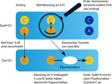
Quantum teleportation via quantum gates is shown in the following two sketches schematically and as a circuit diagram consisting of CNOT, Hadamard and XZ gates [1,2]:

The goal of quantum teleportation is to transfer the state of QuBit C to another QuBit B. Due to the No-Cloning theorem it is however not possible to directly transfer the state of QuBit C to another QuBit without changing the state of QuBit C. The state of QuBit C is initially |QC>:

∣QC⟩=α∣0⟩+β∣1⟩ \Ket{Q_C}=\alpha\Ket{0}+\beta\Ket{1}∣QC​⟩=α∣0⟩+β∣1⟩

Therefore three QuBits are required for the execution of a quantum teleportation: QuBit C has the state to be transferred and the other two entangled QuBits (A and B) are used to transfer the state from QuBit C to QuBit B.

Sequence of a quantum teleportation

  1. Two QuBits A and B are entangled with each other. Bob keeps QuBit B and sends QuBit A to Alice.
  2. Alice concatenates her QuBit C with the received QuBit A via a CNOT gate and applies an Hadamard gate.
  3. Alice measures the states of QuBit C and QuBit A.
  4. Alice communicates the result of the measurements -encoded by two classical bits- via a classical communication channel.
  5. Depending on the measurement result Bob applies X and/or Z gates to his QuBit B to obtain the original state of QuBit C.

Mathematical description of step 1

The entanglement of QuBit A and B yields:

∣e⟩=12(∣00⟩+∣11⟩)=12(∣0⟩A∣0⟩B+∣1⟩A∣1⟩B) \Ket{e}=\frac{1}{\sqrt{2}}(\Ket{00}+\Ket{11})=\frac{1}{\sqrt{2}}(\Ket{0}_{A}\Ket{0}_{B}+\Ket{1}_{A}\Ket{1}_{B}) ∣e⟩=2​1​(∣00⟩+∣11⟩)=2​1​(∣0⟩A​∣0⟩B​+∣1⟩A​∣1⟩B​)

Thus together with QuBit C whose one-particle state is to be transferred, the state vector of the total system at 1. is given by:

∣QC⟩⊗∣e⟩=12(α∣000⟩+α∣011⟩+β∣100⟩+β∣111⟩) \Ket{Q_C}\otimes\Ket{e}=\frac{1}{\sqrt{2}}(\alpha\Ket{000}+\alpha\Ket{011}+\beta\Ket{100}+\beta\Ket{111}) ∣QC​⟩⊗∣e⟩=2​1​(α∣000⟩+α∣011⟩+β∣100⟩+β∣111⟩)

Excursus: Description of the evolution of the total system.

In order to obtain a mathematical expression for the description of the evolution of the total system starting from the quantum gates used so far, we first investigate a system with two QuBits. We consider the case where QuBit q1 experiences a Hadamard gate while QuBit q0 is left undisturbed [3]:


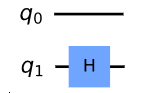
No changes at QuBit q0 are described via the identity matrix I:
I=[1001] I=\begin{bmatrix} 1 & 0\\ 0 & 1 \end{bmatrix} I=[10​01​]
Matrix G that changes the state vector of both QuBits according to the above circuit is obtained from a tensor product of the matrices I and H:
G=I⊗H=[H00H]=12[[11001−1000011001−1]] G=I\otimes H=\begin{bmatrix} H & 0\\ 0 & H \end{bmatrix}=\frac{1}{\sqrt{2}} \Biggl[ \begin{bmatrix} 1 & 1 & 0 & 0\\ 1 & -1 & 0 & 0 \\ 0 & 0 & 1 & 1 \\ 0 & 0 & 1 & -1 \end{bmatrix} \Biggr] G=I⊗H=[H0​0H​]=2​1​[​1100​1−100​0011​001−1​​]

For the used ordering of the entries in the state vector, G is obtained by taking the corresponding matrices in the circuit from top to bottom and combining them from left to right via a tensor product.

Mathematical description of step 2 and explanation of steps 3 and 4

Analogous to the case above with the QuBits q0 and q1, a description of the interaction of QuBit C with QuBit A via a CNOT gate is obtained from a tensor product between the matrices CNOT and I:
G1=CNOT⊗I=[[I0000I00000I00I0]] G_1 = CNOT\otimes I = \Biggl[\begin{bmatrix} I & 0 & 0 & 0\\ 0 & I & 0 & 0 \\ 0 & 0 & 0 & I \\ 0 & 0 & I & 0 \end{bmatrix} \Biggr] G1​=CNOT⊗I=[​I000​0I00​000I​00I0​​]
The description of the subsequent application of a Hadamard gate to QuBit C is obtained from the tensor product between the matrices H, I and I:
G2=12[[I0I00I0II0−I00I0−I]] G_2 = \frac{1}{\sqrt{2}}\Biggl[ \begin{bmatrix} I & 0 & I & 0\\ 0 & I & 0 & I \\ I & 0 & -I & 0 \\ 0 & I & 0 & -I \end{bmatrix} \Biggr] G2​=2​1​[​I0I0​0I0I​I0−I0​0I0−I​​]
The state vector of the total system at 2. is obtained by applying G2G1 (normal matrix product!) to the state vector of the total system at 1.:
(G2⋅G1)(∣QC⟩⊗∣e⟩)=12(H⊗I⊗I)⋅(CNOT⊗I)(α∣000⟩+α∣011⟩+β∣100⟩+β∣111⟩)=12(H⊗I⊗I)(α∣000⟩+α∣011⟩+β∣101⟩+β∣110⟩)=12(α(∣000⟩+∣011⟩+∣100⟩+∣111⟩)+β(∣001⟩+∣010⟩−∣101⟩−∣110⟩))=12(∣00⟩(α∣0⟩+β∣1⟩)+∣01⟩(α∣1⟩+β∣0⟩)+∣10⟩(α∣0⟩−β∣1⟩)+∣11⟩(α∣1⟩−β∣0⟩)) (G_2 \cdot G_1) (\Ket{Q_C} \otimes \Ket{e}) = \\ \frac{1}{\sqrt{2}} (H \otimes I \otimes I) \cdot (CNOT \otimes I) (\alpha\Ket{000}+\alpha\Ket{011}+\beta\Ket{100} + \beta\Ket{111}) = \\ \frac{1}{\sqrt{2}} (H \otimes I \otimes I) (\alpha\Ket{000} + \alpha\Ket{011} + \beta\Ket{101} + \beta\Ket{110}) = \\ \frac{1}{2}(\alpha(\Ket{000} + \Ket{011} + \Ket{100} + \Ket{111}) + \beta(\Ket{001} + \Ket{010} - \Ket{101} - \Ket{110})) = \\ \frac{1}{2}(\color{green}{\Ket{00}}\color{black}{(}\color{blue}{\alpha\Ket{0} + \beta\Ket{1}}\color{black}{)+} \color{green}{\Ket{01}}\color{black}{(}\color{blue}{\alpha\Ket{1} + \beta\Ket{0}}\color{black}{)+}\color{green}{\Ket{10}}\color{black}{(}\color{blue}{\alpha\Ket{0}-\beta\Ket{1}}\color{black}{)+}\color{green}{\Ket{11}}\color{black}{(}\color{blue}{\alpha\Ket{1} - \beta\Ket{0}}\color{black}{))} (G2​⋅G1​)(∣QC​⟩⊗∣e⟩)=2​1​(H⊗I⊗I)⋅(CNOT⊗I)(α∣000⟩+α∣011⟩+β∣100⟩+β∣111⟩)=2​1​(H⊗I⊗I)(α∣000⟩+α∣011⟩+β∣101⟩+β∣110⟩)=21​(α(∣000⟩+∣011⟩+∣100⟩+∣111⟩)+β(∣001⟩+∣010⟩−∣101⟩−∣110⟩))=21​(∣00⟩(α∣0⟩+β∣1⟩)+∣01⟩(α∣1⟩+β∣0⟩)+∣10⟩(α∣0⟩−β∣1⟩)+∣11⟩(α∣1⟩−β∣0⟩))

In the next step Alice performs a measurement on each of her two QuBits C and A. After the measurements she has one of the four states marked in green in the above equation with equal probability (25%). Alice sends the measurement result encoded in two classical bits to Bob, whose QuBit B assumes the corresponding state marked in blue due to the measurement:

Measurement result C, A (Alice) Qubit states |QC QA> after measurement (Alice) QuBit state |QB> after measurment (Bob)
0,0 |00〉 α|0〉+β|1〉
0,1 |01〉 α|1〉+β|0〉
1,0 |10〉 α|0〉-β|1〉
1,1 |11〉 α|1〉-β|0〉

Step 5: X and Z gates

Only in case of the measurement result 0,0 Bobs QuBit B directly takes the original state of QuBit C. In the other three cases, it is necessary to manipulate the state of QuBit B using the X and Z gates in order to recover the original state of QuBit C:

The X gate inverts the state from |0〉to |1〉and vice versa [1]:

The Z gate results in a change of state |+〉to |-〉or |-〉to |+〉[1]:

By using these gates Bob is able to recover the original state of QuBit C in his QuBit B. The following table shows which gates have to be applied to QuBit B depending on the measurement result:

Measurement result C, A (Alice) required gates for QuBit B (Bob)
0,0 none
0,1 X
1,0 Z
1,1 ZX

Excursus: Mathematical representation of the X and Z gates.

The X gate is a simple 2×2 matrix. In this example the X gate changes the QuBit state |0〉to |1〉:
X=[0110],∣0⟩=[10],X∣0⟩=[0110][10]=[01] X=\begin{bmatrix} 0 & 1\\ 1 & 0 \end{bmatrix}, \Ket{0}=\begin{bmatrix} 1\\0 \end{bmatrix}, X\Ket{0}=\begin{bmatrix} 0 & 1\\ 1 & 0 \end{bmatrix}\begin{bmatrix} 1\\ 0 \end{bmatrix}=\begin{bmatrix} 0\\ 1 \end{bmatrix} X=[01​10​],∣0⟩=[10​],X∣0⟩=[01​10​][10​]=[01​]

Also the Z gate is a simple 2×2 matrix. Shown is the change of |+> to |->:
Z=[100−1],∣+⟩=12[11],Z∣+⟩=[100−1]12[11]=12[1−1]=∣−⟩ Z=\begin{bmatrix} 1 & 0\\ 0 & -1 \end{bmatrix}, \Ket{+}=\frac{1}{\sqrt{2}}\begin{bmatrix} 1\\ 1 \end{bmatrix}, Z\Ket{+}=\begin{bmatrix} 1 & 0\\ 0 & -1 \end{bmatrix}\frac{1}{\sqrt{2}}\begin{bmatrix} 1\\ 1 \end{bmatrix}=\frac{1}{\sqrt{2}}\begin{bmatrix} 1\\ -1\end{bmatrix}=\Ket{-} Z=[10​0−1​],∣+⟩=2​1​[11​],Z∣+⟩=[10​0−1​]2​1​[11​]=2​1​[1−1​]=∣−⟩

Sources

[1] M. Ellerhoff. Mit Quanten Rechnen. ISBN 978-3-658-31221-3
[2] P. Kaufmann, S. Naegele-Jackson. II. Quantenrevolution – die Welt der Qubits. In: DFN Mitteilungen Issue 99, June 2021
[3] ibm. Qiskit Textbook. https://github.com/qiskit-community/qiskit-textbook


Version: 18.06.2024

Deutsches Forschungsnetz

DFN-Logo
  • Contact
  • Imprint
  • Privacy
  • Accessibility
  • RSS Feed
Up
Privacy Settings

Our website uses cookies and similar technologies.

Some cookies are necessary for visiting this website, i.e. essential. Otherwise, without these cookies, your end device would not be able to remember your privacy choices, for example.

If you agree, we also use cookies and data to measure your interactions with our website or to integrate external media (e.g. videos).

You can view and withdraw your consent at any time at Privacy policy. On the site you will also find additional information about the cookies and technologies used.

Privacy Settings

Accept all

Save

Accept only essential cookies

Individual privacy settings

Imprint Privacy policy Accessibility

Privacy Settings

Here you will find an overview of all cookies used. You can give your consent to whole categories or display further information and select certain cookies.

Accept all Save Accept only essential cookies

Back

Privacy Settings

Essential cookies enable basic functions and are necessary for the proper function of the website.

Show Cookie Information Hide Cookie Information

Name
Provider Owner of this website
Purpose Saves the visitors preferences selected in the Consent Banner.
Privacy Policy https://www.win-labor.dfn.de/en/privacy/
Hosts www.win-labor.dfn.de
Cookie Name rrze-legal-consent
Cookie Expiry 1 Year
Name
Provider No transmission to third parties
Purpose Test if cookie can be set. Remember User session.
Privacy Policy https://www.win-labor.dfn.de/en/privacy/
Hosts .www.win-labor.dfn.de
Cookie Name wordpress_[*]
Cookie Expiry Session
Name
Provider No transmission to third parties
Purpose Used to manage WebSSO session state.
Privacy Policy https://www.win-labor.dfn.de/en/privacy/
Hosts www.win-labor.dfn.de
Cookie Name SimpleSAMLSessionID,SimpleSAMLAuthToken
Cookie Expiry Session
Name
Provider No transmission to third parties
Purpose Preserves user session state across page requests.
Privacy Policy https://www.win-labor.dfn.de/en/privacy/
Hosts www.win-labor.dfn.de
Cookie Name PHPSESSID
Cookie Expiry Session

Content from video platforms and social media platforms is blocked by default. If External Media cookies are accepted, access to those contents no longer requires manual consent.

Show Cookie Information Hide Cookie Information

Accept
Name
Provider Twitter International Company, One Cumberland Place, Fenian Street, Dublin 2, D02 AX07, Ireland
Purpose Used to unblock Twitter content.
Privacy Policy https://twitter.com/privacy
Hosts twimg.com, twitter.com
Cookie Name __widgetsettings, local_storage_support_test
Cookie Expiry Unlimited
Accept
Name
Provider Google Ireland Limited, Gordon House, Barrow Street, Dublin 4, Ireland
Purpose Used to unblock YouTube content.
Privacy Policy https://policies.google.com/privacy?hl=en&gl=en
Hosts google.com, youtube.com, youtube-nocookie.com
Cookie Name NID
Cookie Expiry 6 Months
Accept
Name
Provider Vimeo Inc., 555 West 18th Street, New York, New York 10011, USA
Purpose Used to unblock Vimeo content.
Privacy Policy https://vimeo.com/privacy
Hosts player.vimeo.com
Cookie Name vuid
Cookie Expiry 2 Years
Accept
Name
Provider Scribd, Inc., 460 Bryant St, 100, San Francisco, CA 94107-2594 USA
Purpose Used to unblock Slideshare content.
Privacy Policy https://www.slideshare.net/privacy
Hosts www.slideshare.net
Cookie Name __utma
Cookie Expiry 2 Years

Imprint Privacy policy Accessibility